本文译自 Implementing a CNN for Text Classification in Tensorflow .
本文我们将实现和Kim Yoon用CNN对句子分类相似的模型。论文中给出的模型在许多文本分类任务(如情感分析)都取得了好的分类表现,并且已经成为了新的文本分类架构的标准baseline。
本文假设你对应用在NLP的CNNs基础知识已经比较熟悉,如果不是,建议先读一下Understanding Convolutional Neural Networks for NLP,以了解必要的背景知识。
Data and Preprocessing
本文使用的数据集是 Movie Review data from Rotten Tomatoes – 原始的论文中也使用的数据之一。该数据集包含了10,662个示例评论句子,一半正向,一半负向。词汇表的大小大约有20k。注意因为该数据集非常小,我们用太强大的模型很可能会过拟合。该数据集也没有用正规的train/test分割,我们简单地使用数据集的10%作为验证集。原始的论文给出的结果在数据集上使用了10-fold交叉验证。
本文不再重复数据预处理的代码,在Github上可以直接获得,预处理主要做了下面几件事:
- 从原始数据文件中加载正负向句子。
- 用和原始论文相同的代码清理文本数据。
- 填充每个句子到的最大句子长度,该数据集上是59。我们添加特殊的\
- 构建词汇表索引,然后将每个词映射到一个0~18765(词汇表的大小)之间的整数。每个句子都成为一个整数向量。
The Model
本文构建的网络看起来大致如下: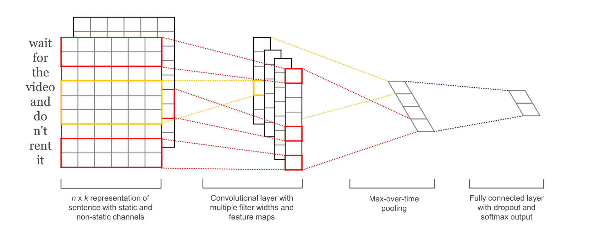
第一层将words嵌入到低维的向量。下一层使用多个filters在嵌入的词向量中做卷积,比如,一次滑动3,4,5个words。然后 max-pool 卷积层的结果到一个长的特征向量,加入dropout正则,使用softmax层对结果进行分类。
本文对原始论文中的模型进行了简化:
- 我们不用预训练好的 word2vec 向量作为我们的word embeddings,而是从头开始学习embeddings。
- 我们不对权重向量做L2正则化限制。对CNNs做句子分类的敏感性分析发现限制会对最终的结果有一点影响。
- 原始论文使用了两个输入数据通道,静态的和非静态的词向量。我们只用一个通道。
It is relatively straightforward (a few dozen lines of code) to add the above extensions to the code here. Take a look at the exercises at the end of the post.
Implementation
为了进行多个超参配置,我们把代码放到TextCNN类中,然后在init函数中生成模型图。
class TextCNN(object):
    """
    CNN进行文本分类
    使用embedding layer,a convolutional, max-pooling 和 softmax layer.
    """
    def __init__(self, sequence_length, num_classes, vocab_size,
                 embedding_size, filter_sizes, num_filters):
为了初始化类,我们需要传递如下参数:
- sequence_length: 句子的长度,我们把所有的句子都填充成了相同的长度(该数据集是59)。
- num_classes: 输出层的类别数,我们这个例子是2(正向和负向)。
- vocab_size: 我们词汇表的大小。定义 embedding 层的大小的时候需要这个参数,embedding层的形状是[vocabulary_size, embedding_size]。
- embedding_size: 嵌入的维度。
- filter_sizes: 我们想要 convolutional filters 覆盖的words的个数,对于每个size,我们会有 num_filters 个 filters。比如 [3,4,5] 表示我们有分别滑过3,4,5个 words 的 filters,总共是3 * num_filters 个 filters。
- num_filters: 每一个filter size的filters数量(见上面)。
Input Placeholders
我们从定义传递给网络的输入数据开始:
# 输入,输出,和dropout的占位符
self.input_x = tf.placeholder(tf.int32, [None, sequence_length], name='input_x')
self.input_y = tf.placeholder(tf.float32, [None, num_classes], name='input_y')
self.dropout_keep_prob = tf.placeholder(tf.float32, name='dropout_keep_prob')
tf.placeholder 创建了一个占位符变量,当我们在训练或者测试运行代码的时候,会把该变量喂给网络。第二个参数是输入张量积的形状。None表示那一维的长度可以是任何值。在这里第一个维度是批大小,使用None表示允许网络处理任意大小的批。
在dropout层保持的神经元的数量也是网络的输入,因为我们可以只在训练过程中启动dropout,而评估模型的时候不启动。
Embedding Layer
我们定义的首层是embedding layer,它将词汇表的词索引映射到低维向量表示。它基本上是我们从数据中学习到的lookup table。
with tf.device('/cpu:0'), tf.name_scope('embedding'):
    W = tf.Variable(tf.random_normal([vocab_size, embedding_size]), name='W')
    self.embedded_chars = tf.nn.embedding_lookup(W, self.input_x)
    self.embedded_chars_expanded = tf.expand_dims(self.embedded_chars, -1)  #扩展维度,在最后一行加1,表示一个通道
We’re using a couple of new features here so let’s go over them:
- tf.device(“/cpu:0”): 强制操作运行在CPU上。 如果有GPU,TensorFlow 会默认尝试把操作运行在GPU上,但是embedding实现目前没有GPU支持,如果使用GPU会报错。
- tf.name_scope: 这个 scope 添加所有的操作到一个叫做“embedding”的高阶节点,使得在TensorBoard可视化你的网络时,你可以得到一个好的层次。
W是训练过程中学习的embedding矩阵,我们用一个随机的均匀分布初始化它。tf.nn.embedding_lookup创建实际的embedding操作。embedding操作的结果是形状为 [None, sequence_length, embedding_size] 的3维张量积。
TensorFlow的卷积conv2d操作接收一个4维的张量,维度分别代表batch, width, height 和 channel。我们的embedding结果不包含 channel 维度,因此我们要手动添加,然后得到形状为[None, sequence_length, embedding_size, 1]的embedding层。
参数说明:TensorFlow中的conv2d定义如下:
def conv2d(input, filter, strides, padding, use_cudnn_on_gpu=None,
           data_format=None, name=None):
  r"""Computes a 2-D convolution given 4-D `input` and `filter` tensors.

  Given an input tensor of shape `[batch, in_height, in_width, in_channels]`
  and a filter / kernel tensor of shape
  `[filter_height, filter_width, in_channels, out_channels]`, this op
  performs the following:
- input: [batch, in_height, in_width, in_channels]
- filter: [filter_height, filter_width, in_channels, out_channels]
[sequence_length, embedding_size] 就是本文前面的那个图中显示的句子的 n x k 表示。
假如使用 size 为 i 的 filter,则该filter的大小为[i, k],经过feature map之后的向量是[n-i+1, 1]。假如共有num_filters_total = num_filters * len(filter_size)个filters,则一个句子(n x k)经过卷积层(feature map)之后变成[num_filters_total, n-i+1, 1]的形状。然后进行max pooling,结果就变成[num_filters_total, 1, 1],最后经过softmax函数即可。
Convolution and Max-Pooling Layers
现在我们准备构建convolutional layers,然后进行max-pooling。注意我们使用不同大小的filters。因为每个卷积会产生不同形状的张量积,我们需要通过他们迭代,为每一个卷积构建一个卷积层,然后把结果合并为一个大的特征向量。
# Create a convolution + maxpool layer for each filter size
pooled_outputs = []
for i, filter_size in enumerate(filter_sizes):
    with tf.name_scope("conv-maxpool-%s" % filter_size):
        # Convolution Layer
        filter_shape = [filter_size, embedding_size, 1, num_filters]
        W = tf.Variable(tf.truncated_normal(filter_shape, stddev=0.1), name="W")
        b = tf.Variable(tf.constant(0.1, shape=[num_filters]), name="b")
        conv = tf.nn.conv2d(
            self.embedded_chars_expanded,
            W,
            strides=[1,1,1,1],
            padding='VALID',
            name='conv')
        # Apply nonlinearity
        h = tf.nn.relu(tf.nn.bias_add(conv, b), name="relu")
        # Max-pooling over the outputs
        pooled = tf.nn.max_pool(
            h,
            ksize = [1, sequence_length-filter_size + 1, 1, 1],
            strides=[1,1,1,1],
            padding='VALID',
            name='pool')
        pooled_outputs.append(pooled)

# Combine all the pooled features
num_filters_total = num_filters * len(filter_size)
self.h_pool = tf.concat(3, pooled_outputs)
self.h_pool_flat = tf.reshape(self.h_pool, [-1, num_filters_total])
这里,W是filter矩阵,h是对卷积输出应用非线性的结果(就是说卷积层用的是relu激活函数),每个filter都在整个embedding上滑动,但是覆盖的words个数不同。”VALID” 填充意味着我们在句子上滑动filter没有填充边缘,做的是narrow convolution,可以得到形状为 [1, sequence_length - filter_size + 1, 1, 1]的输出。对特定的filter大小的输出进行max-pooling得到的是形状为[batch_size, 1, 1, num_filters]的张量积,这基本是一个特征向量,最后的维度对应特征。一旦我们从每个filter size得到了所有的pool了的输出张量积,我们可以将它们结合在一起形成一个长的特征向量,形状是[batch_size, num_filters_total]。在 tf.reshape中使用-1是告诉TensorFlow把维度展平。
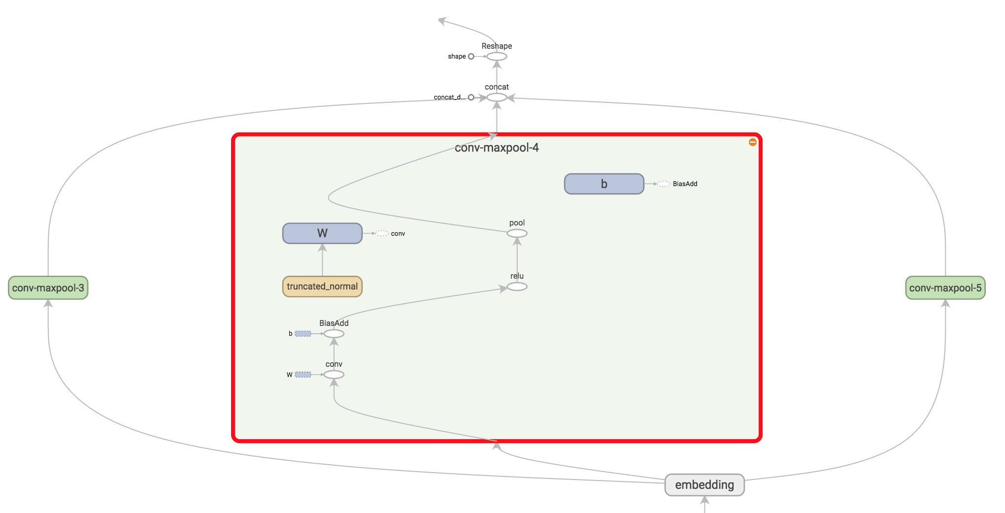
花点时间来理解每一个操作的输出形状。你也可以退回到Understanding Convolutional Neural Networks for NLP再加深一下理解。在TensorBoard中可视化这些操作也是有帮助的(filter大小为3,4和5):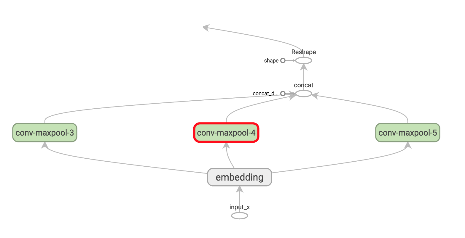
Dropout Layer
Dropout或许是正则化CNNs的最流行的方法。dropout背后的思想是简单的。dropout层随机地屏蔽一部分神经元。这防止神经元一起变化,并且强迫它们单独学习有用的特征。我们激活的部分神经元是通过dropout_keep_prob定义的。在训练期间,我们给它设置一个值,比如0.5,然后在评价的时候设为1(不启动dropout)。
Scores and Predictions
使用经过max-pooling (with dropout applied)的特征向量,我们可以通过做矩阵乘积,然后选择得分最高的类别进行预测。我们也可以应用softmax函数把原始的分数转化为规范化的概率,但是这不会改变我们最终的预测结果。
with tf.name_scope('output'):
            W = tf.Variable(tf.truncated_normal([num_filters_total, num_classes],stddev=0.1), name="W")
            b = tf.Variable(tf.constant(0.1, shape=[num_classes]), name="b")
            self.scores = tf.nn.xw_plus_b(self.h_drop, W, b, name="scores")
            self.predictions = tf.argmax(self.scores, 1, name="predictions")
这里,tf.nn.xw_plus_b 是进行 \(Wx+b\) 矩阵乘积的方便形式。
Loss and Accuracy
使用scores,我们可以定义损失函数。损失是网络犯错的度量,我们的目标是减小它。分类问题的标准损失函数是cross-entropy loss。
# Calculate mean cross-entropy loss
with tf.name_scope("loss"):
    losses = tf.nn.softmax_cross_entropy_with_logits(self.scores, self.input_y)
    self.loss = tf.reduce_mean(losses)
这里 tf.nn.softmax_cross_entropy_with_logits 是一个很方便的函数,可以对给定了分数和正确的输出类别的每个类,计算交叉熵损失。然后我们得到损失的均值。我们也可以用和,但是它很难比较不同批大小和train/dev数据之间的损失。
We also define an expression for the accuracy, which is a useful quantity to keep track of during training and testing.
# Calculate Accuracy
with tf.name_scope("accuracy"):
    correct_predictions = tf.equal(self.predictions, tf.argmax(self.input_y, 1))
    self.accuracy = tf.reduce_mean(tf.cast(correct_predictions, "float"), name="accuracy")
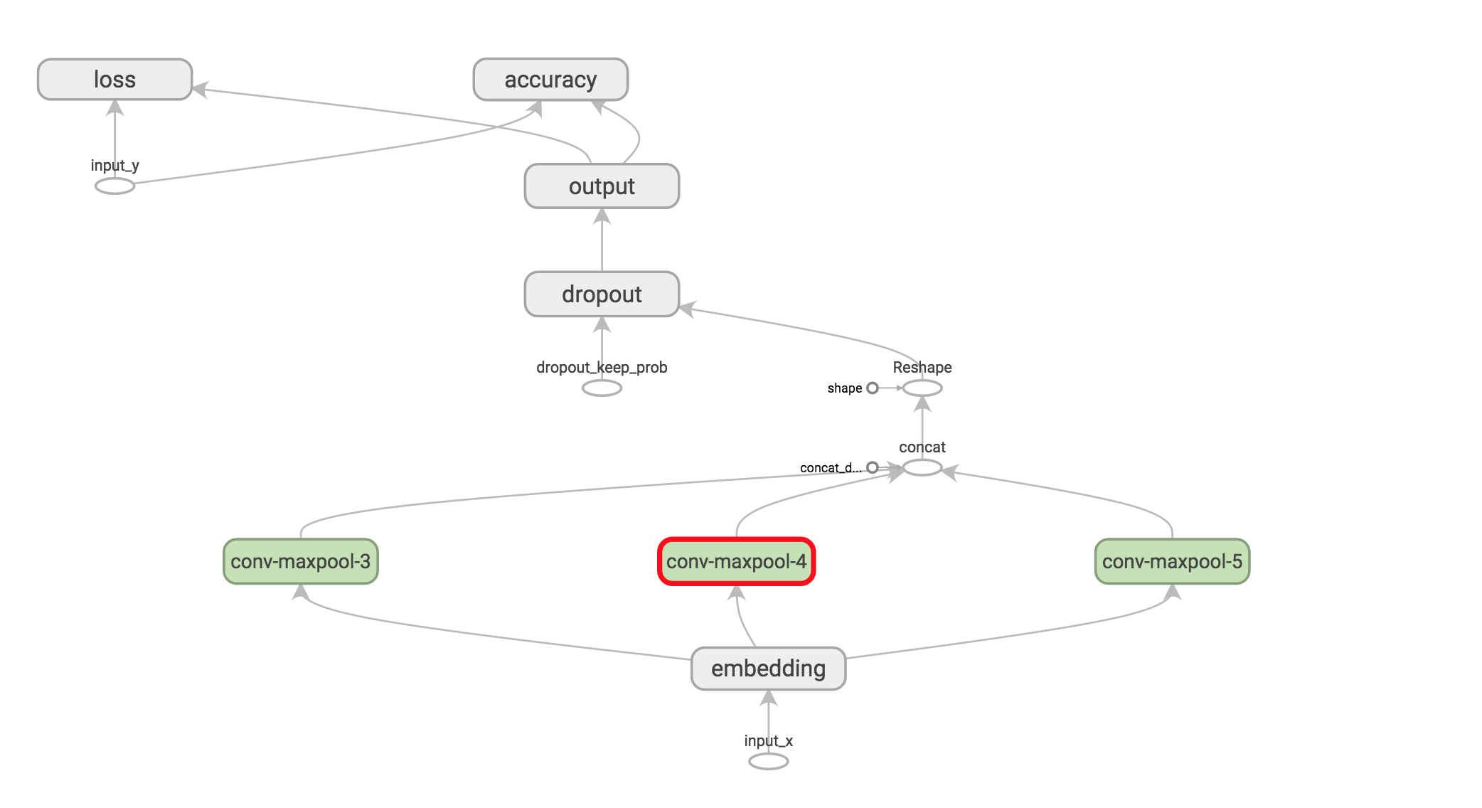
Visualizing the Network
我们已经完成了网络的定义,网络定义的所有代码在这里。为了得到整个蓝图,我们也可以用 TensorBoard 可视化网络: